NumPy for Performance
Please open notebook rsepython-s6r3.ipynb
NumPy constructors
We saw previously that NumPy’s core type is the ndarray, or N-Dimensional Array:
import numpy as np
np.zeros([3,4,2,5])[2,:,:,1]
array([[ 0., 0.],
[ 0., 0.],
[ 0., 0.],
[ 0., 0.]])
The real magic of numpy arrays is that most python operations are applied, quickly, on an element-wise basis.
For example:
x = np.arange(0, 256, 4).reshape(8, 8)
y=np.zeros((8, 8))
%%timeit
for i in range(8):
    for j in range(8):
        y[i][j] = x[i][j] + 10
10000 loops, best of 3: 46.8 µs per loop
x + 10
array([[ 10, 14, 18, 22, 26, 30, 34, 38],
[ 42, 46, 50, 54, 58, 62, 66, 70],
[ 74, 78, 82, 86, 90, 94, 98, 102],
[106, 110, 114, 118, 122, 126, 130, 134],
[138, 142, 146, 150, 154, 158, 162, 166],
[170, 174, 178, 182, 186, 190, 194, 198],
[202, 206, 210, 214, 218, 222, 226, 230],
[234, 238, 242, 246, 250, 254, 258, 262]])
Numpy’s mathematical functions also happen this way, and are said to be “vectorized” functions.
np.sqrt(x)
array([[ 0. , 2. , 2.82842712, 3.46410162,
4. , 4.47213595, 4.89897949, 5.29150262],
[ 5.65685425, 6. , 6.32455532, 6.63324958,
6.92820323, 7.21110255, 7.48331477, 7.74596669],
[ 8. , 8.24621125, 8.48528137, 8.71779789,
8.94427191, 9.16515139, 9.38083152, 9.59166305],
[ 9.79795897, 10. , 10.19803903, 10.39230485,
10.58300524, 10.77032961, 10.95445115, 11.13552873],
[ 11.3137085 , 11.48912529, 11.66190379, 11.83215957,
12. , 12.16552506, 12.32882801, 12.489996 ],
[ 12.64911064, 12.80624847, 12.9614814 , 13.11487705,
13.26649916, 13.41640786, 13.56465997, 13.7113092 ],
[ 13.85640646, 14. , 14.14213562, 14.28285686,
14.4222051 , 14.56021978, 14.69693846, 14.83239697],
[ 14.96662955, 15.09966887, 15.23154621, 15.3622915 ,
15.49193338, 15.62049935, 15.74801575, 15.87450787]])
Numpy contains many useful functions for creating matrices. In our earlier readings we’ve seen linspace and arange for evenly spaced numbers.
np.linspace(0, 10, 21)
array([ 0. , 0.5, 1. , 1.5, 2. , 2.5, 3. , 3.5, 4. ,
4.5, 5. , 5.5, 6. , 6.5, 7. , 7.5, 8. , 8.5,
9. , 9.5, 10. ])
np.arange(0, 10, 0.5)
array([ 0. , 0.5, 1. , 1.5, 2. , 2.5, 3. , 3.5, 4. , 4.5, 5. ,
5.5, 6. , 6.5, 7. , 7.5, 8. , 8.5, 9. , 9.5])
Here’s one for creating matrices like coordinates in a grid:
xmin = -1.5
ymin = -1.0
xmax = 0.5
ymax = 1.0
resolution = 300
xstep = (xmax - xmin) / resolution
ystep = (ymax - ymin) / resolution

ymatrix, xmatrix = np.mgrid[ymin:ymax:ystep, xmin:xmax:xstep]
print(ymatrix)
[[-1. -1. -1. …, -1. -1. -1. ]
[-0.99333333 -0.99333333 -0.99333333 …, -0.99333333 -0.99333333
-0.99333333]
[-0.98666667 -0.98666667 -0.98666667 …, -0.98666667 -0.98666667
-0.98666667]
…,
[ 0.98 0.98 0.98 …, 0.98 0.98 0.98 ]
[ 0.98666667 0.98666667 0.98666667 …, 0.98666667 0.98666667
0.98666667]
[ 0.99333333 0.99333333 0.99333333 …, 0.99333333 0.99333333
0.99333333]]
We can add these together to make a grid containing the complex numbers we want to test for membership in the Mandelbrot set.
values = xmatrix + 1j * ymatrix
print(values)
[[-1.50000000-1.j -1.49333333-1.j -1.48666667-1.j …,
0.48000000-1.j 0.48666667-1.j 0.49333333-1.j ]
[-1.50000000-0.99333333j -1.49333333-0.99333333j -1.48666667-0.99333333j
…, 0.48000000-0.99333333j 0.48666667-0.99333333j
0.49333333-0.99333333j]
[-1.50000000-0.98666667j -1.49333333-0.98666667j -1.48666667-0.98666667j
…, 0.48000000-0.98666667j 0.48666667-0.98666667j
0.49333333-0.98666667j]
…,
[-1.50000000+0.98j -1.49333333+0.98j -1.48666667+0.98j …,
0.48000000+0.98j 0.48666667+0.98j 0.49333333+0.98j ]
[-1.50000000+0.98666667j -1.49333333+0.98666667j -1.48666667+0.98666667j
…, 0.48000000+0.98666667j 0.48666667+0.98666667j
0.49333333+0.98666667j]
[-1.50000000+0.99333333j -1.49333333+0.99333333j -1.48666667+0.99333333j
…, 0.48000000+0.99333333j 0.48666667+0.99333333j
0.49333333+0.99333333j]]
Arraywise Algorithms
We can use this to apply the mandelbrot algorithm to whole ARRAYS
z0 = values
z1 = z0 * z0 + values
z2 = z1 * z1 + values
z3 = z2 * z2 + values
print(z3)
[[ 24.06640625+20.75j 23.16610231+20.97899073j
22.27540349+21.18465854j …, 11.20523832 -1.88650846j
11.57345330 -1.6076251j 11.94394738 -1.31225596j]
[ 23.82102149+19.85687829j 22.94415031+20.09504528j
22.07634812+20.31020645j …, 10.93323949 -1.5275283j
11.28531994 -1.24641067j 11.63928527 -0.94911594j]
[ 23.56689029+18.98729242j 22.71312709+19.23410533j
21.86791017+19.4582314j …, 10.65905064 -1.18433756j
10.99529965 -0.90137318j 11.33305161 -0.60254144j]
…,
[ 23.30453709-18.14090998j 22.47355537-18.39585192j
21.65061048-18.62842771j …, 10.38305264 +0.85663867j
10.70377437 +0.57220289j 11.02562928 +0.27221042j]
[ 23.56689029-18.98729242j 22.71312709-19.23410533j
21.86791017-19.4582314j …, 10.65905064 +1.18433756j
10.99529965 +0.90137318j 11.33305161 +0.60254144j]
[ 23.82102149-19.85687829j 22.94415031-20.09504528j
22.07634812-20.31020645j …, 10.93323949 +1.5275283j
11.28531994 +1.24641067j 11.63928527 +0.94911594j]]
So can we just apply our mandel1 function to the whole matrix?
def mandel1(position,limit=50):
    value = position
    while abs(value) < 2:
        limit -= 1
        value = value**2 + position
        if limit < 0:
            return 0
    return limit
mandel1(values)
—————————————————————————
ValueError Traceback (most recent call last)
—-> 1 mandel1(values)
1 def mandel1(position,limit=50):
2 value=position
—-> 3 while abs(value)<2:
4 limit-=1
5 value=value**2+position
ValueError: The truth value of an array with more than one element is ambiguous. Use a.any() or a.all()
No. The logic of our current routine would require stopping for some elements and not for others.
We can ask numpy to vectorise our method for us:
mandel2 = np.vectorize(mandel1)
data5 = mandel2(values)
from matplotlib import pyplot as plt
%matplotlib inline
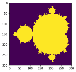
plt.imshow(data5, interpolation='none')
<matplotlib.image.AxesImage at 0x7faad3c74cf8>

Is that any faster?
%%timeit
data5 = mandel2(values)
1 loop, best of 3: 675 ms per loop
This is not significantly faster. When we use vectorize it’s just hiding an plain old python for loop under the hood. We want to make the loop over matrix elements take place in the “C Layer”.
What if we just apply the Mandelbrot algorithm without checking for divergence until the end:
def mandel_numpy_explode(position, limit=50):
    value = position
    while limit > 0:
        limit -= 1
        value = value**2 + position
        diverging = abs(value) > 2


    return abs(value) < 2
data6 = mandel_numpy_explode(values)
/usr/local/lib/python3.5/site-packages/ipykernel/main.py:6: RuntimeWarning: overflow encountered in absolute
/usr/local/lib/python3.5/site-packages/ipykernel/main.py:5: RuntimeWarning: overflow encountered in square
/usr/local/lib/python3.5/site-packages/ipykernel/main.py:5: RuntimeWarning: invalid value encountered in square
/usr/local/lib/python3.5/site-packages/ipykernel/main.py:6: RuntimeWarning: invalid value encountered in greater
/usr/local/lib/python3.5/site-packages/ipykernel/main.py:9: RuntimeWarning: invalid value encountered in less
OK, we need to prevent it from running off to
def mandel_numpy(position, limit=50):
    value = position
    while limit > 0:
        limit -= 1
        value = value**2 + position
        diverging = abs(value) > 2
        # Avoid overflow
        value[diverging] = 2

    return abs(value) < 2
data6 = mandel_numpy(values)
%%timeit

data6 = mandel_numpy(values)
10 loops, best of 3: 58.7 ms per loop
from matplotlib import pyplot as plt
%matplotlib inline
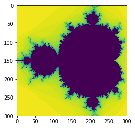
plt.imshow(data6, interpolation='none')
<matplotlib.image.AxesImage at 0x7faad3c15470>
Wow, that was TEN TIMES faster.
There’s quite a few NumPy tricks there, let’s remind ourselves of how they work:
diverging = abs(z3) > 2
z3[diverging] = 2
When we apply a logical condition to a NumPy array, we get a logical array.
x = np.arange(10)
y = np.ones([10]) * 5
z = x > y
x
array([0, 1, 2, 3, 4, 5, 6, 7, 8, 9])
y
array([ 5., 5., 5., 5., 5., 5., 5., 5., 5., 5.])
print(z)
[False False False False False False True True True True]
Logical arrays can be used to index into arrays:
x[x > 3]
array([4, 5, 6, 7, 8, 9])
x[np.logical_not(z)]
array([0, 1, 2, 3, 4, 5])
And you can use such an index as the target of an assignment:
x[z] = 5
x
array([0, 1, 2, 3, 4, 5, 5, 5, 5, 5])
Note that we didn’t compare two arrays to get our logical array, but an array to a scalar integer – this was broadcasting again.
More Mandelbrot
Of course, we didn’t calculate the number-of-iterations-to-diverge, just whether the point was in the set.
Let’s correct our code to do that:
def mandel4(position,limit=50):
    value = position
    diverged_at_count = np.zeros(position.shape)
    while limit > 0:
        limit -= 1
        value = value**2 + position
        diverging = abs(value) > 2
        first_diverged_this_time = np.logical_and(diverging,
                                                  diverged_at_count == 0)
        diverged_at_count[first_diverged_this_time] = limit
        value[diverging] = 2

    return diverged_at_count
data7 = mandel4(values)
plt.imshow(data7, interpolation='none')
<matplotlib.image.AxesImage at 0x7faad3b7aa20>

%%timeit

data7 = mandel4(values)
10 loops, best of 3: 74 ms per loop
Note that here, all the looping over mandelbrot steps was in Python, but everything below the loop-over-positions happened in C.
The code was amazingly quick compared to pure Python.
Can we do better by avoiding a square root?
def mandel5(position, limit=50):
    value = position
    diverged_at_count = np.zeros(position.shape)
    while limit > 0:
        limit -= 1
        value = value**2 + position
        diverging = value * np.conj(value) > 4
        first_diverged_this_time = np.logical_and(diverging, diverged_at_count == 0)
        diverged_at_count[first_diverged_this_time] = limit
        value[diverging] = 2

    return diverged_at_count
%%timeit

data8 = mandel5(values)
10 loops, best of 3: 95.8 ms per loop
Probably not worth the time I spent thinking about it!
NumPy Testing
Now, let’s look at calculating those residuals, the differences between the different datasets.
data8 = mandel5(values)
data5 = mandel2(values)
np.sum((data8 - data5)**2)
0.0
For our non-numpy datasets, numpy knows to turn them into arrays:
xmin = -1.5
ymin = -1.0
xmax = 0.5
ymax = 1.0
resolution = 300
xstep = (xmax-xmin)/resolution
ystep = (ymax-ymin)/resolution
xs = [(xmin + (xmax - xmin) * i / resolution) for i in range(resolution)]
ys = [(ymin + (ymax - ymin) * i / resolution) for i in range(resolution)]
data1 = [[mandel1(complex(x, y)) for x in xs] for y in ys]
sum(sum((data1 - data7)**2))
0.0
But this doesn’t work for pure non-numpy arrays
data2 = []
for y in ys:
    row = []
    for x in xs:
        row.append(mandel1(complex(x, y)))
    data2.append(row)
data2 - data1
—————————————————————————
TypeError Traceback (most recent call last)
—-> 1 data2-data1
TypeError: unsupported operand type(s) for -: ‘list’ and ‘list’
So we have to convert to NumPy arrays explicitly:
sum(sum((np.array(data2) - np.array(data1))**2))
0
NumPy provides some convenient assertions to help us write unit tests with NumPy arrays:
x = [1e-5, 1e-3, 1e-1]
y = np.arccos(np.cos(x))
y
array([ 1.00000004e-05, 1.00000000e-03, 1.00000000e-01])
np.testing.assert_allclose(x, y, rtol=1e-6, atol=1e-20)
np.testing.assert_allclose(data7, data1)
Arraywise operations are fast
Note that we might worry that we carry on calculating the mandelbrot values for points that have already diverged.
def mandel6(position, limit=50):
    value = np.zeros(position.shape) + position
    calculating = np.ones(position.shape, dtype='bool')
    diverged_at_count = np.zeros(position.shape)
    while limit > 0:
        limit -= 1
        value[calculating] = value[calculating]**2 + position[calculating]
        diverging_now = np.zeros(position.shape, dtype='bool')
        diverging_now[calculating] = value[calculating] * \
                                     np.conj(value[calculating])>4
        calculating = np.logical_and(calculating,
                                     np.logical_not(diverging_now))
        diverged_at_count[diverging_now] = limit

    return diverged_at_count
data8 = mandel6(values)
%%timeit

data8 = mandel6(values)
10 loops, best of 3: 60.8 ms per loop
plt.imshow(data8, interpolation='none')
<matplotlib.image.AxesImage at 0x7faad2cfa0b8>
This was not faster even though it was doing less work
This often happens: on modern computers, branches (if statements, function calls) and memory access is usually the rate-determining step, not maths.
Complicating your logic to avoid calculations sometimes therefore slows you down. The only way to know is to measure
Indexing with arrays
We’ve been using Boolean arrays a lot to get access to some elements of an array. We can also do this with integers:
x = np.arange(64)
y = x.reshape([8, 8])
y
array([[ 0, 1, 2, 3, 4, 5, 6, 7],
[ 8, 9, 10, 11, 12, 13, 14, 15],
[16, 17, 18, 19, 20, 21, 22, 23],
[24, 25, 26, 27, 28, 29, 30, 31],
[32, 33, 34, 35, 36, 37, 38, 39],
[40, 41, 42, 43, 44, 45, 46, 47],
[48, 49, 50, 51, 52, 53, 54, 55],
[56, 57, 58, 59, 60, 61, 62, 63]])
y[[2, 5]]
array([[16, 17, 18, 19, 20, 21, 22, 23],
[40, 41, 42, 43, 44, 45, 46, 47]])
y[[0, 2, 5], [1, 2, 7]]
array([ 1, 18, 47])
We can use a : to indicate we want all the values from a particular axis:
y[0:4:2, [0, 2]]
array([[ 0, 2],
[16, 18]])
We can mix array selectors, boolean selectors, :s and ordinary array seqeuencers:
z=x.reshape([4, 4, 4])
z
array([[[ 0, 1, 2, 3],
[ 4, 5, 6, 7],
[ 8, 9, 10, 11],
[12, 13, 14, 15]],
[[16, 17, 18, 19],
[20, 21, 22, 23],
[24, 25, 26, 27],
[28, 29, 30, 31]],
[[32, 33, 34, 35],
[36, 37, 38, 39],
[40, 41, 42, 43],
[44, 45, 46, 47]],
[[48, 49, 50, 51],
[52, 53, 54, 55],
[56, 57, 58, 59],
[60, 61, 62, 63]]])
z[:, [1, 3], 0:3]
array([[[ 4, 5, 6],
[12, 13, 14]],
[[20, 21, 22],
[28, 29, 30]],
[[36, 37, 38],
[44, 45, 46]],
[[52, 53, 54],
[60, 61, 62]]])
We can manipulate shapes by adding new indices in selectors with np.newaxis:
z[:, np.newaxis, [1, 3], 0].shape
(4, 1, 2)
When we use basic indexing with integers and : expressions, we get a view on the matrix so a copy is avoided:
a = z[:, :, 2]
a[0,0] = -500
z
array([[[ 0, 1, -500, 3],
[ 4, 5, 6, 7],
[ 8, 9, 10, 11],
[ 12, 13, 14, 15]],
[[ 16, 17, 18, 19],
[ 20, 21, 22, 23],
[ 24, 25, 26, 27],
[ 28, 29, 30, 31]],
[[ 32, 33, 34, 35],
[ 36, 37, 38, 39],
[ 40, 41, 42, 43],
[ 44, 45, 46, 47]],
[[ 48, 49, 50, 51],
[ 52, 53, 54, 55],
[ 56, 57, 58, 59],
[ 60, 61, 62, 63]]])
We can also use … to specify “: for as many as possible intervening axes”:
z[1]
array([[16, 17, 18, 19],
[20, 21, 22, 23],
[24, 25, 26, 27],
[28, 29, 30, 31]])
z[...,2]
array([[ 2, 6, 10, 14],
[18, 22, 26, 30],
[34, 38, 42, 46],
[50, 54, 58, 62]])
However, boolean mask indexing and array filter indexing always causes a copy.
Let’s try again at avoiding doing unnecessary work by using new arrays containing the reduced data instead of a mask:
def mandel7(position, limit=50):
    positions = np.zeros(position.shape) + position
    value = np.zeros(position.shape) + position
    indices = np.mgrid[0:values.shape[0], 0:values.shape[1]]
    diverged_at_count = np.zeros(position.shape)
    while limit > 0:
        limit -= 1
        value = value**2 + positions
        diverging_now = value * np.conj(value) > 4
        diverging_now_indices = indices[:, diverging_now]
        carry_on = np.logical_not(diverging_now)

        value = value[carry_on]
        indices = indices[:, carry_on]
        positions = positions[carry_on]
        diverged_at_count[diverging_now_indices[0,:],
                          diverging_now_indices[1,:]] = limit

    return diverged_at_count
data9 = mandel7(values)
plt.imshow(data9, interpolation='none')
<matplotlib.image.AxesImage at 0x7faad2cd6588>

%%timeit

data9 = mandel7(values)
10 loops, best of 3: 72.1 ms per loop
Still slower. Probably due to lots of copies – the point here is that you need to experiment to see which optimisations will work. Performance programming needs to be empirical.
Profiling
We’ve seen how to compare different functions by the time they take to run. However, we haven’t obtained much information about where the code is spending more time. For that we need to use a profiler. IPython offers a profiler through the %prun magic. Let’s use it to see how it works:
%prun mandel7(values)
31 function calls in 0.082 seconds
Ordered by: internal time
ncalls tottime percall cumtime percall filename:lineno(function)
1 0.080 0.080 0.082 0.082
1 0.001 0.001 0.002 0.002 index_tricks.py:162(getitem)
1 0.001 0.001 0.001 0.001 numeric.py:1800(indices)
3 0.001 0.000 0.001 0.000 {built-in method numpy.core.multiarray.zeros}
1 0.000 0.000 0.082 0.082 {built-in method builtins.exec}
2 0.000 0.000 0.000 0.000 {built-in method numpy.core.multiarray.arange}
1 0.000 0.000 0.000 0.000 {built-in method numpy.core.multiarray.empty}
1 0.000 0.000 0.082 0.082
2 0.000 0.000 0.000 0.000 {method ‘reshape’ of ‘numpy.ndarray’ objects}
2 0.000 0.000 0.000 0.000 {built-in method math.ceil}
10 0.000 0.000 0.000 0.000 {built-in method builtins.isinstance}
2 0.000 0.000 0.000 0.000 {method ‘append’ of ‘list’ objects}
3 0.000 0.000 0.000 0.000 {built-in method builtins.len}
1 0.000 0.000 0.000 0.000 {method ‘disable’ of ‘_lsprof.Profiler’ objects}
%prun shows a line per each function call ordered by the total time spent on each of these. However, sometimes a line-by-line output may be more helpful. For that we can use the line_profiler package (you need to install it using pip). Once installed you can activate it in any notebook by running:
%load_ext line_profiler
And the %lprun magic should be now available:
%lprun -f mandel7 mandel7(values)
Total time: 0.084526 s
File:
Function: mandel7 at line 1
Line # Hits Time Per Hit % Time Line Contents
==============================================================
1 def mandel7(position, limit=50):
2 1 1654.0 1654.0 2.0 positions = np.zeros(position.shape) + position
3 1 568.0 568.0 0.7 value = np.zeros(position.shape) + position
4 1 1256.0 1256.0 1.5 indices = np.mgrid[0:values.shape[0], 0:values.shape[1]]
5 1 34.0 34.0 0.0 diverged_at_count = np.zeros(position.shape)
6 51 52.0 1.0 0.1 while limit > 0:
7 50 36.0 0.7 0.0 limit -= 1
8 50 9399.0 188.0 11.1 value = value**2 + positions
9 50 14534.0 290.7 17.2 diverging_now = value * np.conj(value) > 4
10 50 5823.0 116.5 6.9 diverging_now_indices = indices[:, diverging_now]
11 50 1565.0 31.3 1.9 carry_on = np.logical_not(diverging_now)
12
13 50 5299.0 106.0 6.3 value = value[carry_on]
14 50 37871.0 757.4 44.8 indices = indices[:, carry_on]
15 50 5452.0 109.0 6.5 positions = positions[carry_on]
16 diverged_at_count[diverging_now_indices[0,:],
17 50 983.0 19.7 1.2 diverging_now_indices[1,:]] = limit
18
19 1 0.0 0.0 0.0 return diverged_at_count
Here, it is clearer to see which operations are keeping the code busy.
Next: Reading - Cython