Performance programming

Please open notebook rsepython-s6r1.ipynb

We’ve spent most of this course looking at how to make code readable and reliable. For research work, it is often also important that code is efficient: that it does what it needs to do quickly.

It is very hard to work out beforehand whether code will be efficient or not: it is essential to Profile code, to measure its performance, to determine what aspects of it are slow.

When we looked at Functional programming, we claimed that code which is conceptualised in terms of actions on whole data-sets rather than individual elements is more efficient. Let’s measure the performance of some different ways of implementing some code and see how they perform.

Two Mandelbrots

You’re probably familiar with a famous fractal called the Mandelbrot Set.

For a complex number $c$, $c$ is in the Mandelbrot set if the series $z_{i+1}=z_{i}^2+c$ (With $z_0=c$) stays close to $0$.

Traditionally, we plot a colour showing how many steps are needed for |$z_i$|$>2$, whereupon we are sure the series will diverge.

Here’s a trivial python implementation:

def mandel1(position, limit=50):

    value = position

    while abs(value) < 2:
        limit -= 1

        value = value**2 + position

        if limit < 0:
            return 0

    return limit

If we run and time our implementation:

xmin=-1.5
ymin=-1.0
xmax=0.5
ymax=1.0
resolution=300
xstep=(xmax-xmin)/resolution
ystep=(ymax-ymin)/resolution
xs=[(xmin+(xmax-xmin)*i/resolution) for i in range(resolution)]
ys=[(ymin+(ymax-ymin)*i/resolution) for i in range(resolution)]

%%timeit
data=[[mandel1(complex(x,y)) for x in xs] for y in ys]

1 loop, best of 3: 705 ms per loop

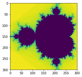
data1=[[mandel1(complex(x,y)) for x in xs] for y in ys]

%matplotlib inline
import matplotlib.pyplot as plt
plt.imshow(data1,interpolation='none')

<matplotlib.image.AxesImage at 0x7fda0311de80>

We will learn in this module how to make a version of this code which works Ten Times faster.

Let’s consider an alternative implementation:

import numpy as np
def mandel_numpy(position,limit=50):
    value = position
    diverged_at_count = np.zeros(position.shape)
    while limit > 0:
        limit -= 1
        value = value**2+position
        diverging = value * np.conj(value) > 4
        first_diverged_this_time = np.logical_and(diverging, diverged_at_count == 0)
        diverged_at_count[first_diverged_this_time] = limit
        value[diverging] = 2

    return diverged_at_count

ymatrix, xmatrix = np.mgrid[ymin:ymax:ystep, xmin:xmax:xstep]

values = xmatrix + 1j*ymatrix

How does this alternative perform?

data_numpy = mandel_numpy(values)

%matplotlib inline
import matplotlib.pyplot as plt
plt.imshow(data_numpy,interpolation='none')

<matplotlib.image.AxesImage at 0x7fda0301a6d8>

%%timeit
data_numpy=mandel_numpy(values)

30.8 ms ± 1.27 ms per loop (mean ± std. dev. of 7 runs, 10 loops each)

Note we get the same answer:

sum(sum(abs(data_numpy-data1)))

0.0

Next: Reading - Faster Mandelbrots?