Scaling for containers and algorithms
Please open notebook rsepython-s6r5.ipynb
We’ve seen that NumPy arrays are really useful. Why wouldn’t we always want to use them for data which is all the same type?
import numpy as np
from timeit import repeat
from matplotlib import pyplot as plt
%matplotlib inline
def time_append_to_ndarray(count):
    # the function repeat does the same that the `%timeit` magic
    # but as a function; so we can plot it.
    return repeat('np.append(before, [0])',
                  f'import numpy as np; before=np.ndarray({count})',
                  number=10000)
def time_append_to_list(count):
    return repeat('before.append(0)',
                  f'before = [0] * {count}',
                  number=10000)
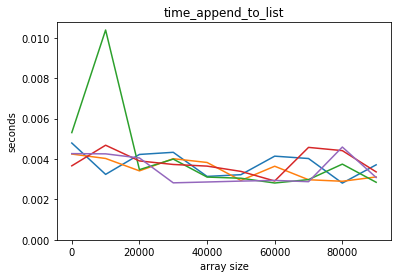
Lets see how fast appending values to a list is
counts = np.arange(1, 100000, 10000)

def plot_time(function, counts, title=None):
    plt.plot(counts, list(map(function, counts)))
    plt.ylim(bottom=0)
    plt.ylabel('seconds')
    plt.xlabel('array size')
    plt.title(title or function.__name__)
plot_time(time_append_to_list, counts)
Compared to appending to a numpy array
plot_time(time_append_to_ndarray, counts)
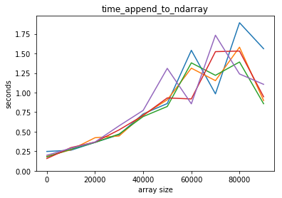
Adding an element to a python list is way faster! Also, it seems that adding an element to a python list is independent of the lenght of the list, but it’s not so for a numpy array.
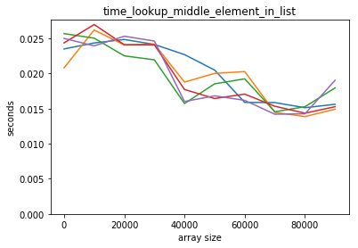
How do they perform when accessing an element on the middle?
def time_lookup_middle_element_in_list(count):
    before = [0] * count
    def totime():
        x = before[count // 2]
    return repeat(totime, number=10000)
def time_lookup_middle_element_in_ndarray(count):
    before=np.ndarray(count)
    def totime():
        x=before[count//2]
    return repeat(totime,number=10000)
def time_lookup_middle_element_in_ndarray(count):
    before = np.ndarray(count)
    def totime():
        x = before[count // 2]
    return repeat(totime, number=10000)
plot_time(time_lookup_middle_element_in_list, counts)
plot_time(time_lookup_middle_element_in_ndarray, counts)
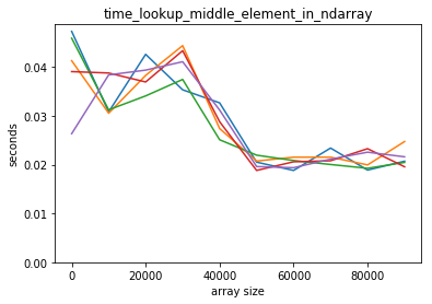
Both scale well for accessing the middle element.
What about inserting at the beginning?
If we want to insert an element at the beginning of a python list we can do:
x = list(range(5))
x
[0, 1, 2, 3, 4]
x[0:0] = [-1]
x
[-1, 0, 1, 2, 3, 4]
def time_insert_to_list(count):
    return repeat('before[0:0]=[0]','before=[0]*'+str(count),number=10000)
def time_insert_to_list(count):
    return repeat('before[0:0] = [0]',
                  f'before = [0] * {count}',number=10000)
plot_time(time_insert_to_list, counts)
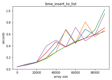
list performs badly for insertions at the beginning!
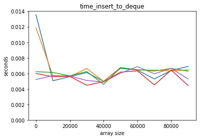
There are containers in Python that work well for insertion at the start:
from collections import deque
def time_insert_to_deque(count):
    return repeat('before.appendleft(0)',
                  f'from collections import deque; before = deque([0] * {count})',
                  number=10000)
plot_time(time_insert_to_deque, counts)
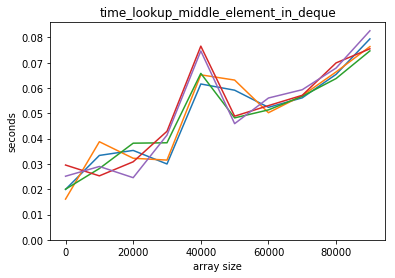
But looking up in the middle scales badly:
def time_lookup_middle_element_in_deque(count):
    before = deque([0] * count)
    def totime():
        x = before[count // 2]
    return repeat(totime, number=10000)
plot_time(time_lookup_middle_element_in_deque, counts)
What is going on here?
Arrays are stored as contiguous memory. Anything which changes the length of the array requires the whole array to be copied elsewhere in memory.
This copy takes time proportional to the array size.
The Python list type is also an array, but it is allocated with extra memory. Only when that memory is exhausted is a copy needed.
Adding an element to a list - memory representation

If the extra memory is typically the size of the current array, a copy is needed every 1/N appends, and costs N to make, so on average copies are cheap. We call this amortized constant time.
The deque type works differently: each element contains a pointer to the next. Inserting elements is therefore very cheap, but looking up the Nth element requires traversing N such pointers.
Adding an element to a deque - memory representation

Dictionary performance
For another example, let’s consider the performance of a dictionary versus a couple of other ways in which we could implement an associative array.
We start by building a dictionary-like class called evildict:
class evildict:
    def __init__(self, data):
        self.data = data

    def __getitem__(self, akey):
        for key, value in self.data:
            if key == akey:
                return value
        raise KeyError()
If we have an eveil dictionary of N elements, how long it would take - on average - to find an element?
eric = [["Name", "Eric Idle"], ["Job", "Comedian"], ["Home", "London"]]
eric_evil = evildict(eric)
eric_evil["Job"]
‘Comedian’
eric_dict = dict(eric)
eric_evil["Job"]
‘Comedian’
x = ["Hello", "License", "Fish", "Eric", "Pet", "Halibut"]
sorted(x, key=lambda el: el.lower())
[‘Eric’, ‘Fish’, ‘Halibut’, ‘Hello’, ‘License’, ‘Pet’]
What if we created a dictionary where we bisect the search?
class sorteddict:
    def __init__(self, data):
        self.data = sorted(data, key = lambda x:x[0])
        self.keys = list(map(lambda x:x[0], self.data))

    def __getitem__(self,akey):
        from bisect import bisect_left
        loc = bisect_left(self.keys, akey)

        if loc != len(self.data):
            return self.data[loc][1]

        raise KeyError()
eric_sorted = sorteddict(eric)
eric_sorted["Job"]
‘Comedian’
This method times the creation of a given dict type and the access of the middle element:
def time_dict_generic(ttype, count, number=10000):
    from random import randrange
    keys = list(range(count))
    values = [0] * count
    data = ttype(list(zip(keys, values)))
    def totime():
        x = data[keys[count // 2]]
    return repeat(totime, number=10000)
time_dict = lambda count: time_dict_generic(dict, count)
time_sorted = lambda count: time_dict_generic(sorteddict, count)
time_evil = lambda count: time_dict_generic(evildict, count)
So we can plot the timing information for each of our three dictionaries.
plot_time(time_sorted, counts, title='sorted')
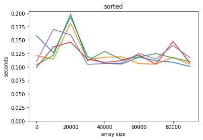
We can’t really see what’s going on here for the sorted example as there’s too much noise, but theoretically we should get logarithmic asymptotic performance.
We write this down as .
This doesn’t mean there isn’t also a constant term, or a term proportional to something that grows slower (such as ): we always write down just the term that is dominant for large .
We saw before that list is for appends, for inserts. Numpy’s array is $O(N)$ for appends.
counts = np.arange(1, 1000, 100)
plot_time(time_evil, counts, title='evil')
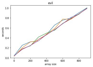
The simple check-each-in-turn solution is $O(N)$ - linear time.
counts = np.arange(1, 100000, 10000)
plot_time(time_dict, counts, title='dict')
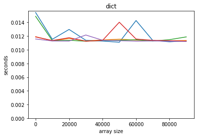
Python’s built-in dictionary is, amazingly, O(1): the time is independent of the size of the dictionary.
This uses a miracle of programming called the Hash Table: you can learn more about these issues at this video from Harvard University. This material is pretty advanced, but, I think, really interesting!
Optional exercise: determine what the asymptotic performance for the Boids model in terms of the number of Boids. Make graphs to support this.
Bonus: how would the performance scale with the number of dimensions?
Return to Modules