Functional Programming
Please open notebook rsepython-s5r2.ipynb
We have previously seen the object-oriented style of programming, and how to organise our code according to it using objects, classes and inheritance. While widely-adopted and very useful, this is not the only way of writing code. The functional paradigm, as the name suggests, emphasises functions as building blocks of programs.
Understanding to think in a functional programming style is almost as important as object orientation for building DRY, clear scientific software, and is just as conceptually difficult.
Functions with Functions
Programs are composed of functions: they take data in (which we call
parameters or arguments) and send data out (through return statements.)
A conceptual trick which is often used by computer scientists to teach the core idea of functional programming is this: to write a program, in theory, you only ever need functions with one argument, even when you think you need two or more. Why?
Let’s define a program to add two numbers:
def add(a, b):
    return a+b

add(5,6)
11
How could we do this, in a fictional version of Python which only defined functions of one argument?
In order to understand this, we’ll have to understand several of the concepts of functional programming.
Let’s start with a program which just adds five to something:
def add_five(a):
    return a+5

add_five(6)
11
OK, we could define lots of these, one for each number we want to add. But that would be infinitely repetitive.
So, let’s try to metaprogram that: we want a function which returns these add_N() functions.
Let’s start with the easy case: a function which returns a function which adds 5 to something:
def generate_five_adder():
    def _add_five(a):
        return a+5
    return _add_five

coolfunction = generate_five_adder()
coolfunction(7)
12
OK, so what happened there? Well, we defined a function inside the other function. We can always do that:
def thirty_function():
    def times_three(a):
        return a*3
    def add_seven(a):
        return a+7
    return times_three(add_seven(3))

thirty_function()
30
When we do this, the functions enclosed inside the outer function are local functions, and can’t be seen outside:
add_seven
—————————————————————————
NameError Traceback (most recent call last)
—-> 1 add_seven
NameError: name ‘add_seven’ is not defined
There’s not really much of a difference between functions and other variables in python.
A function is just a variable which can have () put after it to call the code!
For example, we can do the following:
print(thirty_function)
<function thirty_function at 0x109aabc80>
x=[thirty_function, add_five, add]
for fun in x:
    print(fun)
<function thirty_function at 0x109aabc80>
<function add_five at 0x109aab9d8>
<function add at 0x109aab6a8>
And we know that one of the things we can do with a variable is return it. So we can return a function, and then call it outside:
def deferred_greeting():
    def greet():
        print("Hello")
    return greet

friendlyfunction=deferred_greeting()
# Do something else
print("Just passing the time...")
Just passing the time…
# OK, Go!
friendlyfunction()
Hello
So now, to finish this, we just need to return a function to add an arbitrary amount:
def generate_adder(increment):
    def _adder(a):
        return a + increment
    return _adder

add_3 = generate_adder(3)
add_3(9)
12
We can make this even prettier: let’s make another variable pointing to our generate_adder() function:
add = generate_adder
And now we can do the real magic:
add(8)(5)
13
In summary, we have started with a function that takes two arguments (add(a, b)) and replaced it with a new function (add(a)(b)). This new function takes a single argument, and returns a function that itself takes the second argument.
This may seem like an overly complicated process - and, in some cases, it is! However, this pattern of functions that return functions (or even take them as arguments!) can be very useful. In fact, it is the basis of decorators, a Python feature that we will discuss more in the next reading.
Closures
You may have noticed something a bit weird:
In the definition of generate_adder, increment is a local variable. It should have gone out of scope and died at the end of the definition.
How can the amount the returned adder function is adding still be kept?
This is called a closure.
In Python, whenever a function definition references a variable in the surrounding scope, it is preserved within the function definition.
You can close over global module variables as well:
name = "Jane"

def greet():
    print("Hello, ", name)

greet()
Hello, Jane
And note that the closure stores a reference to the variable in the surrounding scope: (“Late Binding”)
name="Matt"

greet()
Hello, Matt
Map and Reduce
We often want to apply a function to each variable in an array, to return a new array.
We can do this with a list comprehension:
numbers=range(10)

[add_five(i) for i in numbers]
[5, 6, 7, 8, 9, 10, 11, 12, 13, 14]
But this is sufficiently common that there’s a quick built-in function:
list(map(add_five, numbers))
[5, 6, 7, 8, 9, 10, 11, 12, 13, 14]
This map operation is really important conceptually when understanding efficient parallel programming: different computers can apply the mapped function to their input at the same time. We call this Single Program, Multiple Data (SPMD). map is half of the map-reduce functional programming paradigm which is key to the efficient operation of much of today’s “data science” explosion.
Let’s continue our functional programming mind-stretch by looking at reduce operations.
We very often want to loop with some kind of accumulator (an intermediate result that we update), such as when finding a mean:
def summer(data):
    sum = 0.0

    for x in data:
        sum+=x

    return sum
summer(range(10))
45.0
or finding a maximum:
import sys

def my_max(data):
    # Start with the smallest possible number
    highest = sys.float_info.min

    for x in data:
        if x>highest:
            highest=x

    return highest
my_max([2,5,10,-11,-5])
10
These operations, where we have some variable which is building up a result, and the result is updated with some operation, can be gathered together as a functional program, taking in (as an argument) the operation to be used to combine results:
def accumulate(initial, operation, data):
    accumulator=initial
    for x in data:
        accumulator=operation(accumulator, x)
    return accumulator

def my_sum(data):
    def _add(a,b):
        return a+b
    return accumulate(0, _add, data)
my_sum(range(5))
10
Anyway, this accumulate-under-an-operation process is so fundamental to computing that it’s usually in standard libraries for languages which allow functional programming:
def bigger(a,b):
    if b>a:
        return b
    return a

def my_max(data):
    return accumulate(sys.float_info.min, bigger, data)

my_max([2,5,10,-11,-5])
10
Efficient map-reduce
Now, because these operations, _bigger, and _add, are such that e.g. (a+b)+c = a+(b+c) , i.e. they are associative, we could apply our accumulation to the left half and the right half of the array, each on a different computer, and then combine the two halves:
1+2+3+4=(1+2)+(3+4)
Indeed, with a bigger array, we can divide-and-conquer more times:
1+2+3+4+5+6+7+8=((1+2)+(3+4))+((5+6)+(7+8))
So with enough parallel computers, we could do this operation on eight numbers in three steps: first, we use four computers to do one each of the pairwise adds.
Then, we use two computers to add the four totals.
Then, we use one of the computers to do the final add of the two last numbers.
You might be able to do the maths to see that with an N element list, the number of such steps is proportional to the logarithm of N.
We say that with enough computers, reduction operations are O(ln N)
This course isn’t an introduction to algorithms, but we’ll talk more about this O() notation when we think about programming for performance.
Lambda Functions
When doing functional programming, we often want to be able to define a function on the fly:
def most_Cs_in_any_sequence(sequences):

    def count_Cs(sequence):
        return sequence.count('C')

    counts=map(count_Cs, sequences)
    return max(counts)

def most_Gs_in_any_sequence(sequences):
    return max(map(lambda sequence: sequence.count('G'),sequences))

data=[
    "CGTA",
    "CGGGTAAACG",
    "GATTACA"
]

most_Gs_in_any_sequence(data)
4
The syntax here is that these two definitions are identical:
func_name=lambda a,b,c : a+b+c

def func_name(a,b,c):
    return a+b+c
The lambda keyword defines an “anonymous” function.
def most_of_given_base_in_any_sequence(sequences, base):
    return max(map(lambda sequence: sequence.count(base), sequences))

most_of_given_base_in_any_sequence(data,'A')
3
The above fragment defined a lambda function as a closure over base. If you understood that, you’ve got it!
To double all elements in an array:
data=range(10)
list(map(lambda x: 2*x, data))
[0, 2, 4, 6, 8, 10, 12, 14, 16, 18]
[2*x for x in data]
[0, 2, 4, 6, 8, 10, 12, 14, 16, 18]
Similarly, to find the maximum value in a sequence:
def my_max(data): return reduce(lambda a,b: a if a>b else b, data,
        sys.float_info.min)

my_max([2,5,10,-11,-5])
10
Using functional programming for numerical methods
Probably the most common use in research computing for functional programming is the application of a numerical method to a function.
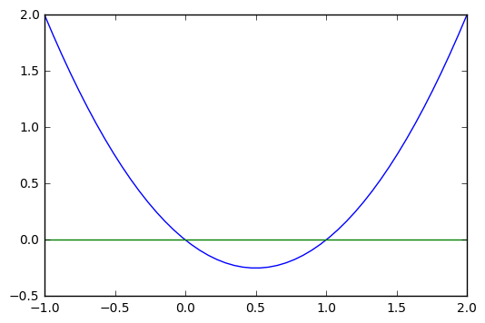
Consider this example which uses the newton function from SciPy, a root-finding function implementing the Newton-Raphson method. The arguments we pass to newton are the function whose roots we want to find, and a starting point to search from.
We will be using this to find the roots of the function .
For example:
% matplotlib inline
from scipy.optimize import newton
from numpy import linspace, zeros
from matplotlib import pyplot as plt

solve_me=lambda x: x**2-x

print(newton(solve_me, 2), newton(solve_me,0.2))

xs=linspace(-1,2,50)
solved=[xs,list(map(solve_me,xs)),xs,zeros(len(xs))]
plt.plot(*solved)
1.0 -3.4419051426429775e-21
[<matplotlib.lines.Line2D at 0x10c09c9e8>,
<matplotlib.lines.Line2D at 0x10c09cc50>]
Sometimes such tools return another function:
def derivative_simple(func, eps, at):
    return (func(at+eps)-func(at))/eps
def derivative(func, eps):
def _func_derived(x):
return (func(x+eps)-func(x))/eps
return _func_derived
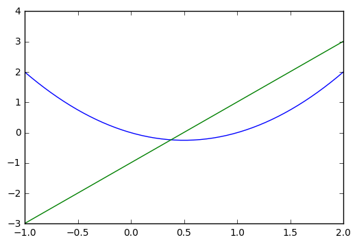
straight = derivative(solve_me, 0.01)
The derivative of solve_me is , which represents a straight line. We can verify that our computations are correct, i.e. that the returned function straight matches , by checking the value of straight at some :
straight(3)
5.00999999999987
or by plotting it:
derived=(xs,list(map(solve_me,xs)),xs,list(map(derivative(solve_me,0.01),xs)))
plt.plot(*derived)
print(newton(derivative(solve_me,0.01),0))
0.49500000000000044
Of course, coding your own numerical methods is bad, because the implementations you develop are likely to be less efficient, less accurate and more error-prone than what you can find in existing established libraries.
For example, the above definition could be replaced by:
import scipy.misc

def derivative(func):
    def _func_derived(x):
        return scipy.misc.derivative(solve_me,x)
    return _func_derived

newton(derivative(solve_me),0)
0.5
If you’ve done a moderate amount of calculus, then you’ll find similarities between functional programming in computer science and Functionals in the calculus of variations.