Numerical Python - NumPy
The Scientific Python Trilogy
Why is Python so popular for research work?
MATLAB has typically been the most popular “language of technical computing”, with strong built-in support for efficient numerical analysis with matrices (the mat in MATLAB is for Matrix, not Maths), and plotting.
Other dynamic languages have cleaner, more logical syntax (Ruby, Scheme)
But Python users developed three critical libraries, matching the power of MATLAB for scientific work:
- Matplotlib, the plotting library created by John D. Hunter
- NumPy, a fast matrix maths library created by Travis Oliphant
- Pandas, data structures and data analysis tools, whose main author is Wes McKinney
- IPython, the precursor of the notebook, created by Fernando Perez
By combining a plotting library, a matrix maths library, and an easy-to-use interface allowing live plotting commands in a persistent environment, the powerful capabilities of MATLAB were matched by a free and open toolchain.
We’ve learned about Matplotlib and Jupyter in this course already. NumPy is the last part of the trilogy.
Limitations of Python Lists
The normal Python List is just one dimensional. To make a matrix, we have to nest Python arrays:
x= [range(5) for something_unused in range(5)]
x
[range(0, 5), range(0, 5), range(0, 5), range(0, 5), range(0, 5)]
Applying an operation to every element is a pain:
x + 5
—————————————————————————
TypeError Traceback (most recent call last)
<ipython-input-3-057023a07318> in <module>()
—-> 1 x + 5
TypeError: can only concatenate list (not “int”) to list
[[elem +5 for elem in row] for row in x]
[[5, 6, 7, 8, 9],
[5, 6, 7, 8, 9],
[5, 6, 7, 8, 9],
[5, 6, 7, 8, 9],
[5, 6, 7, 8, 9]]
Common useful operations like transposing a matrix or reshaping a 10 by 10 matrix into a 20 by 5 matrix are not easy to code in raw Python lists.
The NumPy array
NumPy’s array type represents a multidimensional matrix Mi,j,k…n
The NumPy array seems at first to be just like a list:
import numpy as np
my_array = np.array(range(5))
my_array
array([0, 1, 2, 3, 4])
my_array[2]
2
for element in my_array:
    print("Hello" * element)
Hello
HelloHello
HelloHelloHello
HelloHelloHelloHello
We can also see our first weakness of NumPy arrays versus Python lists:
my_array.append(4)
—————————————————————————
AttributeError Traceback (most recent call last)
<ipython-input-9-ad82621ab44a> in <module>()
—-> 1 my_array.append(4)
AttributeError: ‘numpy.ndarray’ object has no attribute ‘append’
For NumPy arrays, you typically don’t change the data size once you’ve defined your array, whereas for Python lists, you can do this efficiently. However, you get back lots of goodies in return…
Elementwise Operations
But most operations can be applied element-wise automatically!
my_array * 2
array([0, 2, 4, 6, 8])
These “vectorized” operations are very fast: (we can use %%timeit magic )
import numpy as np
big_list = range(10000)
big_array = np.arange(10000)
%%timeit
[x**2 for x in big_list]
3.45 ms ± 7.68 µs per loop (mean ± std. dev. of 7 runs, 100 loops each)
%%timeit
big_array**2
11.8 µs ± 77.3 ns per loop (mean ± std. dev. of 7 runs, 100000 loops each)
Arange and linspace
NumPy has two easy methods for defining floating-point evenly spaced arrays:
x=np.arange(0,10,0.1)
y = list(range(0, 10, 0.1))
—————————————————————————
TypeError Traceback (most recent call last)
—-> 1 y = list(range(0, 10, 0.1))
TypeError: ‘float’ object cannot be interpreted as an integer
We can quickly define non-integer ranges of numbers for graph plotting:
import math
values = np.linspace(0, math.pi, 100) # Start, stop, number of steps
values
array([ 0. , 0.03173326, 0.06346652, 0.09519978, 0.12693304,
0.1586663 , 0.19039955, 0.22213281, 0.25386607, 0.28559933,
0.31733259, 0.34906585, 0.38079911, 0.41253237, 0.44426563,
0.47599889, 0.50773215, 0.53946541, 0.57119866, 0.60293192,
0.63466518, 0.66639844, 0.6981317 , 0.72986496, 0.76159822,
0.79333148, 0.82506474, 0.856798 , 0.88853126, 0.92026451,
0.95199777, 0.98373103, 1.01546429, 1.04719755, 1.07893081,
1.11066407, 1.14239733, 1.17413059, 1.20586385, 1.23759711,
1.26933037, 1.30106362, 1.33279688, 1.36453014, 1.3962634 ,
1.42799666, 1.45972992, 1.49146318, 1.52319644, 1.5549297 ,
1.58666296, 1.61839622, 1.65012947, 1.68186273, 1.71359599,
1.74532925, 1.77706251, 1.80879577, 1.84052903, 1.87226229,
1.90399555, 1.93572881, 1.96746207, 1.99919533, 2.03092858,
2.06266184, 2.0943951 , 2.12612836, 2.15786162, 2.18959488,
2.22132814, 2.2530614 , 2.28479466, 2.31652792, 2.34826118,
2.37999443, 2.41172769, 2.44346095, 2.47519421, 2.50692747,
2.53866073, 2.57039399, 2.60212725, 2.63386051, 2.66559377,
2.69732703, 2.72906028, 2.76079354, 2.7925268 , 2.82426006,
2.85599332, 2.88772658, 2.91945984, 2.9511931 , 2.98292636,
3.01465962, 3.04639288, 3.07812614, 3.10985939, 3.14159265])
NumPy comes with ‘vectorised’ versions of common functions which work element-by-element when applied to arrays:
%matplotlib inline
from matplotlib import pyplot as plt
plt.plot(values, np.sin(values))
[<matplotlib.lines.Line2D at 0x2b89cb146c88>]
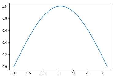
So we don’t have to use awkward list comprehensions when using these.
Multi-Dimensional Arrays
NumPy’s true power comes from multi-dimensional arrays:
np.zeros([3,4,2])
array([[[ 0., 0.],
[ 0., 0.],
[ 0., 0.],
[ 0., 0.]],
[[ 0., 0.],
[ 0., 0.],
[ 0., 0.],
[ 0., 0.]],
[[ 0., 0.],
[ 0., 0.],
[ 0., 0.],
[ 0., 0.]]])
Unlike a list-of-lists in Python, we can reshape arrays:
x=np.array(range(40))
y=x.reshape([4,5,2])
y
array([[[ 0, 1],
[ 2, 3],
[ 4, 5],
[ 6, 7],
[ 8, 9]],
[[10, 11],
[12, 13],
[14, 15],
[16, 17],
[18, 19]],
[[20, 21],
[22, 23],
[24, 25],
[26, 27],
[28, 29]],
[[30, 31],
[32, 33],
[34, 35],
[36, 37],
[38, 39]]])
And index multiple columns at once:
y[3,2,1]
35
Including selecting on inner axes while taking all from the outermost:
y[:,2,1]
array([ 5, 15, 25, 35])
And sub-selecting ranges:
y[2:,:1,:]
array([[[20, 21]],
[[30, 31]]])
And transpose arrays:
y.transpose()
array([[[ 0, 10, 20, 30],
[ 2, 12, 22, 32],
[ 4, 14, 24, 34],
[ 6, 16, 26, 36],
[ 8, 18, 28, 38]],
[[ 1, 11, 21, 31],
[ 3, 13, 23, 33],
[ 5, 15, 25, 35],
[ 7, 17, 27, 37],
[ 9, 19, 29, 39]]])
You can get the dimensions of an array with shape
y.shape
(4, 5, 2)
y.transpose().shape
(2, 5, 4)
Some numpy functions apply by default to the whole array, but can be chosen to act only on certain axes:
x=np.arange(12).reshape(4,3)
x
array([[ 0, 1, 2],
[ 3, 4, 5],
[ 6, 7, 8],
[ 9, 10, 11]])
x.sum(1) # Sum along the second axis, leaving the first.
array([ 3, 12, 21, 30])
x.sum(0) # Sum along the first axis, leaving the second.
array([18, 22, 26])
x.sum() # Sum all axes
66
Array Datatypes
A Python list can contain data of mixed type, can be said to be heterogenous:
x = ['hello', 2, 3.4]
type(x[2])
float
type(x[1])
int
A NumPy array always contains just one datatype, can be said to be homogenous:
np.array(x)
array([‘hello’, ‘2’, ‘3.4’],
dtype=’<U5’)
NumPy will choose the least-generic-possible datatype that can contain the data:
y=np.array([2, 3.4])
y
array([ 2. , 3.4])
type(y[0])
numpy.float64
Broadcasting
This is another really powerful feature of NumPy.
By default, array operations are element-by-element:
np.arange(5) * np.arange(5)
array([ 0, 1, 4, 9, 16])
If we multiply arrays with non-matching shapes we get an error:
np.arange(5) * np.arange(6)
—————————————————————————
ValueError Traceback (most recent call last)
<ipython-input-39-66b7c967724c> in <module>()
—-> 1 np.arange(5) * np.arange(6)
ValueError: operands could not be broadcast together with shapes (5,) (6,)
np.zeros([2,3]) * np.zeros([2,4])
—————————————————————————
ValueError Traceback (most recent call last)
<ipython-input-40-bf6e403cd465> in <module>()
—-> 1 np.zeros([2,3]) * np.zeros([2,4])
ValueError: operands could not be broadcast together with shapes (2,3) (2,4)
m1 = np.arange(100).reshape([10, 10])
m2 = np.arange(100).reshape([10, 5, 2])
m1 + m2
—————————————————————————
ValueError Traceback (most recent call last)
<ipython-input-43-24e1f0a857c4> in <module>()
—-> 1 m1 + m2
ValueError: operands could not be broadcast together with shapes (10,10) (10,5,2)
Arrays must match in all dimensions in order to be compatible:
np.ones([3,3]) * np.ones([3,3]) # Note elementwise multiply, *not* matrix multiply.
« array([[ 1., 1., 1.],
[ 1., 1., 1.],
[ 1., 1., 1.]])
Except, that if one array has any Dimension 1, then the data is REPEATED to match the other.
m1 = np.arange(10).reshape([10,1])
m1
array([[0],
[1],
[2],
[3],
[4],
[5],
[6],
[7],
[8],
[9]])
m2 = m1.transpose()
m2
array([[0, 1, 2, 3, 4, 5, 6, 7, 8, 9]])
m1.shape # "Column Vector"
(10, 1)
m2.shape # "Row Vector"
(1, 10)
m1 + m2
array([[ 0, 1, 2, 3, 4, 5, 6, 7, 8, 9],
[ 1, 2, 3, 4, 5, 6, 7, 8, 9, 10],
[ 2, 3, 4, 5, 6, 7, 8, 9, 10, 11],
[ 3, 4, 5, 6, 7, 8, 9, 10, 11, 12],
[ 4, 5, 6, 7, 8, 9, 10, 11, 12, 13],
[ 5, 6, 7, 8, 9, 10, 11, 12, 13, 14],
[ 6, 7, 8, 9, 10, 11, 12, 13, 14, 15],
[ 7, 8, 9, 10, 11, 12, 13, 14, 15, 16],
[ 8, 9, 10, 11, 12, 13, 14, 15, 16, 17],
[ 9, 10, 11, 12, 13, 14, 15, 16, 17, 18]])
10 * m1 + m2
array([[ 0, 1, 2, 3, 4, 5, 6, 7, 8, 9],
[10, 11, 12, 13, 14, 15, 16, 17, 18, 19],
[20, 21, 22, 23, 24, 25, 26, 27, 28, 29],
[30, 31, 32, 33, 34, 35, 36, 37, 38, 39],
[40, 41, 42, 43, 44, 45, 46, 47, 48, 49],
[50, 51, 52, 53, 54, 55, 56, 57, 58, 59],
[60, 61, 62, 63, 64, 65, 66, 67, 68, 69],
[70, 71, 72, 73, 74, 75, 76, 77, 78, 79],
[80, 81, 82, 83, 84, 85, 86, 87, 88, 89],
[90, 91, 92, 93, 94, 95, 96, 97, 98, 99]])
This works for arrays with more than one unit dimension.
Newaxis
Broadcasting is very powerful, and numpy allows indexing with np.newaxis to temporarily create new one-long dimensions on the fly.
x = np.arange(10).reshape(2,5)
y = np.arange(8).reshape(2,2,2)
x.reshape(2,5,1,1)
array([[[[0]],
[[1]],
[[2]],
[[3]],
[[4]]],
[[[5]],
[[6]],
[[7]],
[[8]],
[[9]]]])
x[:,:,np.newaxis,np.newaxis].shape
(2, 5, 1, 1)
y[:,np.newaxis,:,:].shape
(2, 1, 2, 2)
res = x[:,:,np.newaxis,np.newaxis] * y[:,np.newaxis,:,:]
res.shape
(2, 5, 2, 2)
np.sum(res)
830
Note that newaxis works because a 3 x 1 x 3 array and a 3 x 3 array contain the same data,
differently shaped:
threebythree = np.arange(9).reshape(3,3)
threebythree
array([[0, 1, 2],
[3, 4, 5],
[6, 7, 8]])
threebythree[:, np.newaxis, :]
array([[[0, 1, 2]],
[[3, 4, 5]],
[[6, 7, 8]]])
Dot Products
NumPy multiply is element-by-element, not a dot-product:
a = np.arange(9).reshape(3, 3)
a
array([[0, 1, 2],
[3, 4, 5],
[6, 7, 8]])
b = np.arange(3, 12).reshape(3, 3)
b
array([[3, 4, 5],
[6, 7, 8],
[9, 10, 11]])
a * b
array([[0, 4, 10],
[18, 28, 40],
[54, 70, 88]])
To get a dot-product, (matrix inner product) we can use a built in function:
np.dot(a,b)
array([[24, 27, 30],
[78, 90, 102],
[132, 153, 174]])
Though it is possible to represent this in the algebra of broadcasting and newaxis:
a[:, :, np.newaxis].shape
(3, 3, 1)
b[np.newaxis, :, :].shape
(1, 3, 3)
a[:, :, np.newaxis] * b[np.newaxis, :, :]
array([[[ 0, 0, 0],
[ 6, 7, 8],
[18, 20, 22]],
[[ 9, 12, 15],
[24, 28, 32],
[45, 50, 55]],
[[18, 24, 30],
[42, 49, 56],
[72, 80, 88]]])
(a[:, :, np.newaxis] * b[np.newaxis, :, :]).sum(1)
array([[ 24, 27, 30],
[ 78, 90, 102],
[132, 153, 174]])
Or if you prefer:
(a.reshape(3, 3, 1) * b.reshape(1, 3, 3)).sum(1)
array([[ 24, 27, 30],
[ 78, 90, 102],
[132, 153, 174]])
We use broadcasting to generate $A_{ij}B_{jk}$ as a 3-d matrix:
a.reshape(3, 3, 1) * b.reshape(1, 3, 3)
array([[[ 0, 0, 0],
[ 6, 7, 8],
[18, 20, 22]],
[[ 9, 12, 15],
[24, 28, 32],
[45, 50, 55]],
[[18, 24, 30],
[42, 49, 56],
[72, 80, 88]]])
Then we sum over the middle, $j$ axis, [which is the 1-axis of three axes numbered (0,1,2)] of this 3-d matrix. Thus we generate $\Sigma_j A_{ij}B_{jk}$.
We can see that the broadcasting concept gives us a powerful and efficient way to express many linear algebra operations computationally.
Record Arrays
These are a special array structure designed to match the CSV “Record and Field” model. It’s a very different structure from the normal numPy array, and different fields can contain different datatypes. We saw this when we looked at CSV files:
x = np.arange(50).reshape([10,5])
record_x = x.view(dtype={'names': ["col1", "col2", "another", "more",
                                   "last"],
                         'formats': [int]*5 } )
record_x
array([[(0, 1, 2, 3, 4)],
[(5, 6, 7, 8, 9)],
[(10, 11, 12, 13, 14)],
[(15, 16, 17, 18, 19)],
[(20, 21, 22, 23, 24)],
[(25, 26, 27, 28, 29)],
[(30, 31, 32, 33, 34)],
[(35, 36, 37, 38, 39)],
[(40, 41, 42, 43, 44)],
[(45, 46, 47, 48, 49)]],
dtype=[(‘col1’, ‘<i8’), (‘col2’, ‘<i8’), (‘another’, ‘<i8’), (‘more’, ‘<i8’), (‘last’, ‘<i8’)])
Record arrays can be addressed with field names like they were a dictionary:
record_x['col1']
array([[ 0],
[ 5],
[10],
[15],
[20],
[25],
[30],
[35],
[40],
[45]])
We’ve seen these already when we used NumPy’s CSV parser.
Logical arrays, masking, and selection
Numpy defines operators like == and < to apply to arrays element by element
x = np.zeros([3,4])
x
array([[ 0., 0., 0., 0.],
[ 0., 0., 0., 0.],
[ 0., 0., 0., 0.]])
y = np.arange(-1,2)[:,np.newaxis] * np.arange(-2,2)[np.newaxis,:]
y
array([[ 2, 1, 0, -1],
[ 0, 0, 0, 0],
[-2, -1, 0, 1]])
iszero =  x == y
iszero
array([[False, False, True, False],
[ True, True, True, True],
[False, False, True, False]], dtype=bool)
A logical array can be used to select elements from an array:
y[np.logical_not(iszero)]
array([ 2, 1, -1, -2, -1, 1])
Although when printed, this comes out as a flat list, if assigned to, the selected elements of the array are changed!
y[iszero] = 5
y
array([[ 2, 1, 5, -1], [ 5, 5, 5, 5], [-2, -1, 5, 1]])
Numpy memory
Numpy memory management can be tricksy:
x = np.arange(5)
y = x[:]
y[2] = 0
x
array([0, 1, 0, 3, 4])
It does not behave like lists!
x = list(range(5))
y = x[:]
y[2] = 0
x
[0, 1, 2, 3, 4]
We must use np.copy to force separate memory. Otherwise NumPy tries it’s hardest to make slices be views on data.
Now, this has all been very theoretical, but let’s go through a practical example, and see how powerful NumPy can be.
Next: Reading - The Boids!