Field and Record Data
Let’s carry on with our sunspots example:
import requests
spots = requests.get('http://www.sidc.be/silso/INFO/snmtotcsv.php').text
spots.split('\n')[0]
‘1749;01;1749.042; 96.7; -1.0; -1;1’
We want to work programmatically with Separated Value files.
These are files which have:
- Each record on a line
- Each record has multiple fields
- Fields are separated by some separator
Typical separators are the space, tab, comma, and semicolon separated values files, e.g.:
- Space separated value (e.g.
field1, "field two", field3) - Comma separated value (e.g.
field1, another field, "wow, another field")
Comma-separated-value is abbreviated CSV, and tab separated value TSV.
CSV is also used to refer to all the different sub-kinds of separated value files, i.e. some people use csv to refer to tab, space and semicolon separated files.
CSV is not a particularly superb data format, because it forces your data model to be a list of lists. Richer file formats describe “serialisations” for dictionaries and for deeper-than-two nested list structures as well.
Nevertheless, because you can always export spreadsheets as CSV files, (each cell is a field, each row is a record) CSV files are very popular.
CSV variants.
Some CSV formats define a comment character, so that rows beginning with, e.g., a #, are not treated as data, but give a human index.
Some CSV formats define a three-deep list structure, where a double-newline separates records into blocks.
Some CSV formats assume that the first line defines the names of the fields, e.g.:
name, age, job
Jacob, 38, Postman
Elizabeth, 19, Student
Python CSV readers
The Python standard library has a csv module. However, it’s less powerful than the CSV capabilities in numpy,
the main scientific python library for handling data. Numpy is destributed with Anaconda and Canopy, so we recommend you just use that.
Numpy has powerful capabilities for handling matrices, and other fun stuff, and we’ll learn about these later in the course,
but for now, we’ll just use numpy’s CSV reader, and assume it makes us lists and dictionaries, rather than it’s more exciting
array type.
import numpy as np
import requests
spots = requests.get('http://www.sidc.be/silso/INFO/snmtotcsv.php', stream=True)
stream=True delays loading all of the data until it is required.
sunspots = np.genfromtxt(spots.raw, delimiter=';')
genfromtxt is a powerful CSV reader. I used the delimiter optional argument to specify the delimeter. I could also specify
names=True if I had a first line naming fields, and comments=# if I had comment lines.
sunspots[0][3]
96.7
We can now plot the “Sunspot cycle”:
%matplotlib inline
from matplotlib import pyplot as plt
plt.plot(sunspots[:,0], sunspots[:,3]) # Numpy syntax to access all
                                       #rows, specified column.
[<matplotlib.lines.Line2D at 0x2b0724397da0>]
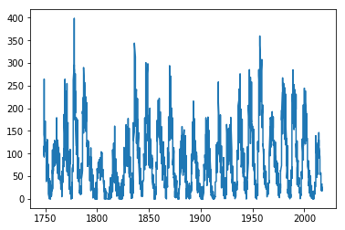
The plot command accepted an array of ‘X’ values and an array of ‘Y’ values. We used a special NumPy “:” syntax, which we’ll learn more about later.
Naming Columns
I happen to know that the columns here are defined as follows:
From http://www.sidc.be/silso/infosnmtot:
CSV
Filename: SN_m_tot_V2.0.csv
Format: Comma Separated values (adapted for import in spreadsheets)
The separator is the semicolon ‘;’.
Contents:
- Column 1-2: Gregorian calendar date
- Year
- Month
- Column 3: Date in fraction of year.
- Column 4: Monthly mean total sunspot number.
- Column 5: Monthly mean standard deviation of the input sunspot numbers.
- Column 6: Number of observations used to compute the monthly mean total sunspot number.
- Column 7: Definitive/provisional marker. ‘1’ indicates that the value is definitive. ‘0’ indicates that the value is still provisional.
I can actually specify this to the formatter:
spots = requests.get('http://www.sidc.be/silso/INFO/snmtotcsv.php', stream=True)

sunspots = np.genfromtxt(spots.raw, delimiter=';',
                         names=['year','month','date',
                         'mean','deviation','observations','definitive'])
sunspots
array([(1749.0, 1.0, 1749.042, 96.7, -1.0, -1.0, 1.0),
(1749.0, 2.0, 1749.123, 104.3, -1.0, -1.0, 1.0),
(1749.0, 3.0, 1749.204, 116.7, -1.0, -1.0, 1.0), …,
(2017.0, 2.0, 2017.122, 26.1, 3.5, 448.0, 0.0),
(2017.0, 3.0, 2017.204, 17.7, 2.6, 884.0, 0.0),
(2017.0, 4.0, 2017.286, 32.6, 3.6, 831.0, 0.0)],
dtype=[(‘year’, ‘<f8’), (‘month’, ‘<f8’), (‘date’, ‘<f8’), (‘mean’, ‘<f8’), (‘deviation’, ‘<f8’), (‘observations’, ‘<f8’), (‘definitive’, ‘<f8’)])
Typed Fields
It’s also often good to specify the datatype of each field.
spots = requests.get('http://www.sidc.be/silso/INFO/snmtotcsv.php', stream=True)

sunspots = np.genfromtxt(spots.raw, delimiter=';',
                         names=['year','month','date',
                         'mean','deviation','observations','definitive'],
                         dtype=[int, int, float, float, float, int, int])
sunspots
array([(1749, 1, 1749.042, 96.7, -1.0, -1, 1),
(1749, 2, 1749.123, 104.3, -1.0, -1, 1),
(1749, 3, 1749.204, 116.7, -1.0, -1, 1), …,
(2017, 2, 2017.122, 26.1, 3.5, 448, 0),
(2017, 3, 2017.204, 17.7, 2.6, 884, 0),
(2017, 4, 2017.286, 32.6, 3.6, 831, 0)],
dtype=[(‘year’, ‘<i8’), (‘month’, ‘<i8’), (‘date’, ‘<f8’), (‘mean’, ‘<f8’), (‘deviation’, ‘<f8’), (‘observations’, ‘<i8’), (‘definitive’, ‘<i8’)])
Now, NumPy understands the names of the columns, so our plot command is more readable:
sunspots['year']
array([1749, 1749, 1749, …, 2017, 2017, 2017])
plt.plot(sunspots['year'],sunspots['mean'])
[<matplotlib.lines.Line2D at 0x2b07243e3b00>]
